CLASSIFICATION Classification with non-neural networks, non-deep learning algorithms

/source of the picture: SuperAI.pl/
Decision Trees Classifier with Scikit-Learn: classification on Iris Dataset
#0. Setup the environment for training, testing, and using SuperAI with chosen machine learning techniques.
        #0A. Open Anaconda.
        #0B. Create and set (if you want) the environment to work in. It must be done only once per preffered settings.
        #0C. Open Jupyter Notebook.
        #0D. Import and use (if you want) the 'warnings' library that is preinstalled with Anaconda to make the ouput cleaner.
        import warnings
        warnings.filterwarnings('ignore')
BASIC INSTALLS
import sklearn
        import graphviz
        import matplotlib
        import pip
        import sys

        print("Python version: {}".format(sys.version))
        print("pip version: {}".format(pip.__version__))
        print("scikit-learn version: {}".format(sklearn.__version__))
        print("graphviz version: {}".format(graphviz.__version__))
        print("matplotlib version: {}".format(matplotlib.__version__))
!pip install scikit-learn==1.5.1
#!pip install graphviz==0.20.1 #doesn't seem to work properly on Windows at the moment
For Windows in the CMD.exe Prompt (from Anaconda) run:
conda install python-graphviz==0.20.1
!pip install matplotlib==3.9.0
import sklearn
        import graphviz
        import matplotlib
        import pip
        import sys

        print("Python version: {}".format(sys.version))
        print("pip version: {}".format(pip.__version__))
        print("scikit-learn version: {}".format(sklearn.__version__))
        print("graphviz version: {}".format(graphviz.__version__))
        print("matplotlib version: {}".format(matplotlib.__version__))
from sklearn.datasets import load_iris
        from sklearn import tree
        iris = load_iris()
        X, y = iris.data, iris.target
        clf = tree.DecisionTreeClassifier()
        clf = clf.fit(X, y)
tree.plot_tree(clf)
import graphviz
        dot_data = tree.export_graphviz(clf, out_file=None)
        graph = graphviz.Source(dot_data)
        graph.render("iris")
dot_data = tree.export_graphviz(clf, out_file=None,
                             feature_names=iris.feature_names,
                             class_names=iris.target_names,
                             filled=True, rounded=True,
                             special_characters=True)
        graph = graphviz.Source(dot_data)
        graph
Checking overall score of the classifier
clf.score(X, y)
Adding train - test split
from sklearn.model_selection import train_test_split
        X_train, X_test, y_train, y_test = train_test_split(X, y, random_state=0)

        clf = tree.DecisionTreeClassifier(random_state=0)
        clf = clf.fit(X_train, y_train)

        clf.score(X_train, y_train)
clf.score(X_test, y_test)
clf.score(X, y)
tree.plot_tree(clf)
import graphviz
        dot_data = tree.export_graphviz(clf, out_file=None)
        graph = graphviz.Source(dot_data)
        graph.render("iris")
dot_data = tree.export_graphviz(clf, out_file=None,
                             feature_names=iris.feature_names,
                             class_names=iris.target_names,
                             filled=True, rounded=True,
                             special_characters=True)
        graph = graphviz.Source(dot_data)
        graph
Used Dataset: Breast Cancer Wisconsin Dataset
Problem to solve / Decision to make: Classification (malignant / benign tumor)
ML Libraries used to solve the problem: Scikit-Learn
ML Methods / Algorithms used to solve the problem: Decision Tree
General info about the used Methods / Algorithms:
You can read more about Decision Trees at:
More info about the Methods/Algorithms + Source of the Example + Source of the Dataset:
We'll use Scikit-Learn, one of the most popular ML libraries. You can read more about using DT with Scikit-Learn (classification and regression) at their website:
And especially you can read about Decision Tree Classifier:
At first we'll see how it works with the dataset from Scikit-Learn pool of datasets:
We want the dataset that is good for classification and with the least possible classes. So we'll use the Breast Cancer Wisconsin Dataset, because it is, in a way, one of the simplest - it has only 2 classes beteween which the algorithms chooses: malignant and benign.
With this dataset we can also see how helpful the machine learning can be in diagnostic medicine. The algorithm will help us to decide wether the tumor that was detected was benign (non-cancerous) or malignant - cancerous. If you want to learn more about difference between benign and malignant tumors you can read or watch about it in the Internet. It's good to know about it.
/source of the picture: SuperAI.pl/
0. Setup the environment for training, testing, and using SuperAI with chosen machine learning techniques.
0A. Open Anaconda.
0B. Create and set (if you want) the environment to work in. It must be done only once per preffered settings.
0C. Open Jupyter Notebook.
0D. Import and use (if you want) the 'warnings' library that is preinstalled with Anaconda to make the ouput cleaner.
1. Install and import all the libraries for machine learning and helper libraries
1A. Install all the necessary libraries not yet installed (must be done only once in one evironment)
1B. Load/Import the libraries for machine learning and helper libraries (check the versions of the libraries)
2. Prepare computer environment for using the model (training, testing, etc.), e.g. set CPU or GPU device for working.
3. Load the data (or create some data for learning purposes, training and testing the model).
4. Check the data: basic description, some examples.
5. Prepare the data for using with the chosen machine learning technique (e.g. normalize pixel values) and recheck the data.
6. Prepare the data for tackling overfitting problem, e. g. divide the data into train, test sets and recheck the data.
7. Create the model (define the model, choose and set the hyperparameters, etc.).
8. Visualize the model (as it is at the moment).
9. Prepare the functions for training and testing the model (if neccessary).
10. Train the model.
11. Test the model (remember to test the model in the evaluation mode (dropouts, batch normalizations, etc.), if applies)
12. Show the specific results and metrics (if you want).
13. Visualize the trained model.
14. Prepare the model for using with one example (prediction, generation, etc.).
15. Check the model with some examples.
{
16. Modify the model (extra step if you want, but it's not neccessary).
17. Test the modified model (extra step, if applies).
} * x
18. Save the trained model.
19. Load and test the saved trained model.
20. Combine all the necessary steps in one SuperAI that will be able to use the model.
21. Check the SuperAI.
And you are ready to use this great SuperAI!
Setting up the work station = Ready to work computer
To start working with this notebook, you need Python and Jupyter Notebook.
To get Python, go to https://www.anaconda.com, download it, and install it.
After you install Anaconda on your computer, create a new environment in it (with 1 click) and install Jupyter Notebook and CMD.exe Prompt within the environment (with 2 clicks). If you don't know how to do it, you can check one of my previous tutorials: Python 101 for Beginners (https://superai.pl/courses/python_101_for_beginners.html).
After you do it, you are ready to start working with this notebook.
So here we are:
|
0. Setup the environment for training, testing, and using SuperAI with chosen machine learning techniques. |
|
|
0A. Open Anaconda. |
|
|
0B. Create and set (if you want) the environment to work in. It must be done only once per preffered settings. |
|
|
0C. Open Jupyter Notebook. |
|
|
0D. Import and use (if you want) the 'warnings' library that is preinstalled with Anaconda to make the ouput cleaner. |
|
|
1. Install and import all the libraries for machine learning and helper libraries |
And here comes the code:
#0. Setup the environment for training, testing, and using SuperAI with chosen machine learning techniques.
        #0A. Open Anaconda.
        #0B. Create and set (if you want) the environment to work in. It must be done only once per preffered settings.
        #0C. Open Jupyter Notebook.
        #0D. Import and use (if you want) the 'warnings' library that is preinstalled with Anaconda to make the ouput cleaner.
        import warnings
        warnings.filterwarnings('ignore')
#1. Install and import all the libraries for machine learning and helper libraries
        #1A. Install all the necessary libraries not yet installed (must be done only once in one evironment)

        #!pip install graphviz --upgrade
        #!pip install pandas --upgrade
        #!pip install pydot --upgrade
        #!pip install scikit-learn --upgrade
#1B. Load/Import the libraries for machine learning and helper libraries (check the versions of the libraries)

        import sklearn
        from sklearn import tree
        from sklearn.datasets import load_breast_cancer
        from sklearn.metrics import confusion_matrix, ConfusionMatrixDisplay
        from sklearn.model_selection import train_test_split
        from sklearn.tree import DecisionTreeClassifier
        from sklearn.tree import export_graphviz

        import graphviz
        import IPython
        from IPython.display import Image
        import matplotlib as mpl
        import matplotlib.pyplot as plt
        import numpy as np
        import os
        import pandas as pd
        import pickle
        import pydot
        import sys

        print("Python version: {}".format(sys.version))
        print("scikit-learn version: {}".format(sklearn.__version__))
        print("graphviz version: {}".format(graphviz.__version__))
        print("IPython version: {}".format(IPython.__version__))
        print("Matplotlib version: {}".format(mpl.__version__))
        print("Numpy version: {}".format(np.__version__))
        print("Pandas version: {}".format(pd.__version__))
        print("pickle version: {}".format(pickle.format_version))
        print("pydot version: {}".format(pydot.__version__))
So, if you want to recreate this environment with the same versions of libraries as I have:
Create an environment with Python version: 3.11.9
Put this into requirements.txt:
scikit-learn==1.5.0
graphviz==0.20.1
IPython==8.20.0
matplotlib==3.9.0
numpy==2.1.0
pandas==2.2.2
pydot==2.0.0
requirements = "requirements.txt"
        with open(requirements, 'w', encoding="utf-8") as f:
            print(
        """scikit-learn==1.5.1
        graphviz==0.20.1
        IPython==8.25.0
        matplotlib==3.9.0
        numpy==2.1.0
        pandas==2.2.2
        pydot==2.0.0""", file=f)
!pip install -r requirements.txt
!pip install -r requirements.txt
#1B. Load/Import the libraries for machine learning and helper libraries (check the versions of the libraries)

        import sklearn
        from sklearn import tree
        from sklearn.datasets import load_breast_cancer
        from sklearn.metrics import confusion_matrix, ConfusionMatrixDisplay
        from sklearn.model_selection import train_test_split
        from sklearn.tree import DecisionTreeClassifier
        from sklearn.tree import export_graphviz

        import graphviz
        import IPython
        from IPython.display import Image
        import matplotlib as mpl
        import matplotlib.pyplot as plt
        import numpy as np
        import os
        import pandas as pd
        import pickle
        import pydot
        import sys

        print("Python version: {}".format(sys.version))
        print("scikit-learn version: {}".format(sklearn.__version__))
        print("graphviz version: {}".format(graphviz.__version__))
        print("IPython version: {}".format(IPython.__version__))
        print("Matplotlib version: {}".format(mpl.__version__))
        print("Numpy version: {}".format(np.__version__))
        print("Pandas version: {}".format(pd.__version__))
        print("pickle version: {}".format(pickle.format_version))
        print("pydot version: {}".format(pydot.__version__))
#2. Prepare computer environment for using the model (training, testing, etc.), e.g. set CPU or GPU device for working.
        # Nothing to do here at the moment.
#3. Load the data (or create some data for learning purposes, training and testing the model).
        breast_cancer_data = load_breast_cancer(as_frame=True)

        X = features = breast_cancer_data.data.copy()
        y = target = breast_cancer_data.target.copy()

        classes = [breast_cancer_data.target_names[0], breast_cancer_data.target_names[1]]
#4. Check the data: basic description, some examples.
        print("There are {} items in {} classes in the dataset to classify tested data into:\n\n\
        0 = {} = {} items = {:.2f}% of the data \n1 = {} = {} items = {:.2f}% of the data".format(len(X), len(classes),
                                                classes[0], target.value_counts()[0],  target.value_counts()[0] / len(target) * 100,
                                                classes[1], target.value_counts()[1], target.value_counts()[1] / len(target) * 100))

        print("\nThere are {} features we can take under consideration:".format(len(breast_cancer_data.feature_names)),
              breast_cancer_data.feature_names)

        print("\nHere is a part of the dataframe with the features based on which we might try to learn how to classify the data:")
        X
print("We check the data:")
        X.info()
print("We check specifically for missing data:")
        X.isnull().sum()
        #X.isna().sum()
print("We show the data:")
        X.hist(bins=50, figsize=(20,15))
        plt.show()
#EXTRA MESSING WITH THE DATA: adding missing data

        X_with_missing = X.copy()
        X_with_missing.iloc[0,0] = np.nan

        print("We've changed mean radius in 0th row (that was: {}) to NaN. Here is the table as it looks now:".format(X.iloc[0,0]))
        X_with_missing
print("Here is the data check:")
        X_with_missing.info()
print("We check for missing data in our dataframe with missing data:")
        X_with_missing.isnull().sum()
#Dropping the rows with missing data

        X_without_missing_dropped_example = X_with_missing.dropna(axis=0)

        print("We've dropped the first row. We have all the columns. Here is the head of the table as it looks now:")

        X_without_missing_dropped_example.head(3)
#EXTRA MESSING WITH THE DATA: adding missing data in 3 columns

        X_with_missing2 = X.copy()
        X_with_missing2.iloc[0,0] = np.nan
        X_with_missing2.iloc[1,1] = np.nan
        X_with_missing2.iloc[2,2] = np.nan

        print("We've changed mean radius in the 0th row, mean texture in the 1st row, and mean parameter in the 2nd row.\
        \nHere is the table as it looks now:")
        X_with_missing2
X_with_missing2 = X_with_missing2.dropna(subset=["mean area"]) #dropping when NA is in particular column, if it's there
        print("We've tried to drop a subset with NAs in mean area, but there wasn't anything to drop so nothig has changed.\
        \nHere is the table as it looks now:")
        X_with_missing2
X_with_missing2 = X_with_missing2.dropna(subset=["mean radius"]) #dropping when NA is in particular column, otherwise do it without subset
        print("We did drop 0th row in a subset with NAs in mean radius, the rest of the table stays the same even with NAs.\
        \nHere is the table as it looks now:")
        X_with_missing2
X_with_missing2 = X_with_missing2.dropna()
        print("We did drop 0th row, 1st row, and 2nd row with all NAs in the table. Here is the table as it looks now:")
        X_with_missing2
#EXTRA: MESSING WITH THE DATA: adding missing data

        X_with_missing = X.copy()
        X_with_missing.iloc[0,0] = np.nan

        print("We've changed mean radius in 0th row (that was: {}) to NaN. Here is the table as it looks now:".format(X.iloc[0,0]))
        X_with_missing
#Dropping the columns with missing data.

        X_without_missing_dropped_column = X_with_missing.dropna(axis=1)

        print("We've dropped the first column. We have all the rows. Here is the table as it looks now:")

        X_without_missing_dropped_column
#EXTRA: MESSING WITH THE DATA: adding missing data in 3 columns

        X_with_missing2 = X.copy()
        X_with_missing2.iloc[0,0] = np.nan
        X_with_missing2.iloc[1,1] = np.nan
        X_with_missing2.iloc[2,2] = np.nan

        print("We've changed mean radius in the 0th row, mean texture in the 1st row, and mean parameter in the 2nd row.\
        \nHere is the table as it looks now:")
        X_with_missing2
X_with_missing2.mean()
X.mean()
#Filling missing data with mean

        X_without_missing_filled_mean = X_with_missing2.fillna(X_with_missing2.mean())

        print("We've changed mean radius in 0th row (that was: {:.2f}) to mean of the rest, that is: {:.6f}. \
        \nHere is the table as it looks now:\n".format(X.iloc[0,0], X_without_missing_filled_mean.iloc[0,0]))

        print("We've changed mean texture in 1st row (that was: {:.2f}) to mean of the rest, that is: {:.6f}. \
        \nHere is the table as it looks now:\n".format(X.iloc[1,1], X_without_missing_filled_mean.iloc[1,1]))

        print("We've changed mean perimeter in 2nd row (that was: {:.2f}) to mean of the rest, that is: {:.6f}. \
        \nHere is the table as it looks now:\n".format(X.iloc[2,2], X_without_missing_filled_mean.iloc[2,2]))

        X_without_missing_filled_mean
#EXTRA: MESSING WITH THE DATA: adding missing data in 3 columns

        X_with_missing2 = X.copy()
        X_with_missing2.iloc[0,0] = np.nan
        X_with_missing2.iloc[1,1] = np.nan
        X_with_missing2.iloc[2,2] = np.nan

        print("We've changed mean radius in the 0th row, mean texture in the 1st row, and mean parameter in the 2nd row. \
        \nHere is the table as it looks now:")
        X_with_missing2
X_with_missing2.median()
#Filling missing data with median

        X_without_missing_filled_median = X_with_missing2.fillna(X_with_missing2.median())

        print("We've changed mean radius in 0th row (that was: {:.2f}) to median of the rest, that is: {:.6f}. \
        \nHere is the table as it looks now:\n".format(X.iloc[0,0], X_without_missing_filled_median.iloc[0,0]))

        print("We've changed mean texture in 1st row (that was: {:.2f}) to median of the rest, that is: {:.6f}. \
        \nHere is the table as it looks now:\n".format(X.iloc[1,1], X_without_missing_filled_median.iloc[1,1]))

        print("We've changed mean perimeter in 2nd row (that was: {:.2f}) to median of the rest, that is: {:.6f}. \
        \nHere is the table as it looks now:\n".format(X.iloc[2,2], X_without_missing_filled_median.iloc[2,2]))

        X_without_missing_filled_median
#Data check
        print("Here is the data check:")
        X_with_missing2.describe()
#Data check
        print("Here is the data check:")
        X_without_missing_filled_median.describe()
print("We can check how the data in the dataframe is distributed to see if there isn't something wrong.\
        \nIt's good to know something about the dataset to decide if there is something wrong or not, like that \
        'mean radius' can't be too different from 'worst radius' or something like this.")
        X.describe()
print("Here is the histogram of the first column: 'mean radius'")
        X.iloc[:,0].hist(bins=100, figsize=(8,6))
print("Here are some plots with first four features:")
        to_plot = pd.DataFrame(X.iloc[:, :4], columns=breast_cancer_data.feature_names[:4])
        pl = pd.plotting.scatter_matrix(to_plot, c=y, alpha=0.5, figsize=(20, 20), marker='.', s=250)
X.plot(kind="scatter", x="fractal dimension error", y="worst fractal dimension", alpha=0.2)
X_with_changed_mean_radius = X.copy()
        X_with_changed_mean_radius.iloc[0,0] = 1111.1

        print("We've changed mean radius in first cell in 0th row that was: {} to extremely different value, that is: {}. \
        \nHere is the table as it looks now:".format(X.iloc[0,0], X_with_changed_mean_radius.iloc[0,0]))

        X_with_changed_mean_radius.head(3)
X_with_changed_mean_radius.describe()
print("Here is the histogram of the first column of the changed: 'mean radius'")
        X_with_changed_mean_radius.iloc[:,0].hist(bins=100, figsize=(8,6))
print("And here are some plots with first four features with the wrong mean radius:")
        to_plot = pd.DataFrame(X_with_changed_mean_radius.iloc[:, :4], columns=breast_cancer_data.feature_names[:4])
        pl = pd.plotting.scatter_matrix(to_plot, c=y, alpha=0.5, figsize=(20, 20), marker='.', s=250)
#Dropping the row with extreme value
        X_with_changed_mean_radius_with_deleted_row = X_with_changed_mean_radius.drop([0], axis=0)

        print("We've droped the row with extreme value and now here is part of the table as it looks now:")

        X_with_changed_mean_radius_with_deleted_row.head(3)
X_with_changed_mean_radius_with_deleted_row.describe()
print("Here is the histogram of the first column of the changed: 'mean radius'")
        X_with_changed_mean_radius_with_deleted_row.iloc[:,0].hist(bins=100, figsize=(8,6))
print("And here are some plots with first four features with the deleted wrong mean radius.")
        print("We need to change the target data first. We do it now by changing c=y to c=y_changed and deleting the first row in it.")

        y_changed = y[1:]

        print("And here are the plots:")
        to_plot = pd.DataFrame(X_with_changed_mean_radius_with_deleted_row.iloc[:, :4], columns=breast_cancer_data.feature_names[:4])
        pl = pd.plotting.scatter_matrix(to_plot, c=y_changed, alpha=0.5, figsize=(20, 20), marker='.', s=250)
If using mean, don't forget to calculate it from non-outliers and save this number, beacuse you might need it in the future.
#Filling with mean or median from others
        X_with_changed_mean_radius_with_mean_from_others = X_with_changed_mean_radius.copy()
        X_with_changed_mean_radius_with_mean_from_others.iloc[0,0] = X_with_changed_mean_radius[1:].mean()[0]
        #X_with_changed_mean_radius_with_mean_from_others.iloc[0,0] = X_with_changed_mean_radius[1:].median()[0]

        print("We've changed mean radius in 0th row (that was: {}) to mean of the rest, that is: {}. \
        \nHere is the table as it looks now:".format(X_with_changed_mean_radius.iloc[0,0], X_with_changed_mean_radius[1:].mean()[0]))

        X_with_changed_mean_radius_with_mean_from_others.head(3)
X_with_changed_mean_radius_with_mean_from_others.describe()
print("Here is the histogram of the first column of the changed: 'mean radius'")
        X_with_changed_mean_radius_with_mean_from_others.iloc[:,0].hist(bins=100, figsize=(8,6))
print("And here are some plots with first four features with the changed mean radius:")
        to_plot = pd.DataFrame(X_with_changed_mean_radius_with_mean_from_others.iloc[:, :4],
                               columns=breast_cancer_data.feature_names[:4])
        pl = pd.plotting.scatter_matrix(to_plot, c=y, alpha=0.5, figsize=(20, 20), marker='.', s=250)
#After-digression data check
        print("Here is the data check:")
        X.info()
#EXTRA: MESSING WITH THE DATA: choosing only some features as the dataset

        chosen_feature1 = "fractal dimension error"
        chosen_feature2 = "worst fractal dimension"
        chosen_features = [chosen_feature1, chosen_feature2]

        X = features = breast_cancer_data.data.copy()[chosen_features]

        print("\nLet's choose only '{}' and '{}' as features to classify the data.".format(chosen_feature1, chosen_feature2))

        print("\nHere is a part of the dataframe with the feature we've chosen to classify the data:")
        X
and
= Prepare the data for using with the chosen machine learning technique (normalize pixel values, deal with categorical data, divide the data into train, validation, test sets, try to have even classes, scale or standarize the data, etc.) and recheck the data.
#5. Prepare the data for using with the chosen machine learning technique (normalize pixel values, deal with categorical data,
        #divide the data into train, validation, test sets, try to have even classes, scale or standarize the data, etc.)
        #and recheck the data.

        X_train, X_test, y_train, y_test = train_test_split(features, target, train_size=0.1, test_size=0.9, random_state = 0)

        print("There are {} items in {} classes in the train dataset to classify tested data into:\n\n\
        0 = {} = {} items = {:.2f}% of the data \n1 = {} = {} items = {:.2f}% of the data".format(len(X_train), len(classes),
                                            classes[0], y_train.value_counts()[0], y_train.value_counts()[0] / len(y_train) * 100,
                                            classes[1], y_train.value_counts()[1], y_train.value_counts()[1] / len(y_train) * 100))

        print("\nThere are {} items in {} classes in the test dataset to classify tested data into:\n\n\
        0 = {} = {} items = {:.2f}% of the data \n1 = {} = {} items = {:.2f}% of the data".format(len(X_test), len(classes),
                                            classes[0], y_test.value_counts()[0], y_test.value_counts()[0] / len(y_test) * 100,
                                            classes[1], y_test.value_counts()[1], y_test.value_counts()[1] / len(y_test) * 100))

        print("\nHere is a part of the dataframe with the features based on which we'll try to learn how to classify the data:")
        X_train
        #X_test
        #y_train
        #y_test
#7. Create the model (define the model, choose and set the hyperparameters, etc.).
        clf = DecisionTreeClassifier(random_state = 0)
#8. Visualize the model (as it is at the moment).
        # Nothing to do here at the moment.
#9. Prepare the functions for training and testing the model (if neccessary).
        # Nothing to do here at the moment.
#10. Train the model.
        #Train the classifier
        clf.fit(X_train, y_train)
#11. Test the model (remember to test the model in the evaluation mode (dropouts, batch normalizations, etc.), if applies)
        #Print results
        print("Training result: {:.3f}".format(clf.score(X_train, y_train)))
        print("Test result: {:.3f}".format(clf.score(X_test, y_test)))

        #Show confusion matrix
        y_true = y_test
        y_pred = clf.predict(X_test)
        cm = confusion_matrix(y_true, y_pred)
        disp = ConfusionMatrixDisplay(confusion_matrix = cm, display_labels = classes)
        disp.plot(cmap="gist_ncar")
#12. Show the specific results and metrics (if you want).
        # Nothing to do here at the moment.
#13. Visualize the trained model.
        #Plot the Decision Tree
        #tree.plot_tree(clf)

        print("There are {} items in {} classes in the train dataset to classify tested data into:\n\n\
        0 = {} = {} items = {:.2f}% of the data \n1 = {} = {} items = {:.2f}% of the data".format(len(X_train), len(classes),
                                            classes[0], y_train.value_counts()[0], y_train.value_counts()[0] / len(y_train) * 100,
                                            classes[1], y_train.value_counts()[1], y_train.value_counts()[1] / len(y_train) * 100))

        print("\nThere are {} features we take under consideration: {}\n".format(len(X_train.columns),
              list(X_train.columns)))

        export_graphviz(clf, out_file="cancer_decision_tree.dot", class_names = ["malignant", "benign"],
                       feature_names=(chosen_features), impurity=False, filled=True)
        os.environ["PATH"] += os.pathsep + 'C:\Program Files\Graphviz\bin'
        with open ("cancer_decision_tree.dot") as f:
            dot_graph = f.read()
        #graphviz.Source(dot_graph)

        (graph,) = pydot.graph_from_dot_file('cancer_decision_tree.dot')
        graph.write_png('cancer_decision_tree.png')
        display(Image(filename='cancer_decision_tree.png'))
n_features = len(chosen_features)
        plt.barh(range(n_features), clf.feature_importances_, align='center')
        plt.yticks(np.arange(n_features), chosen_features)
        plt.xlabel("Feature Importance")
        plt.ylabel("Feature")

        print("Feature Importance: \n{}: {}, \n{}: {}\n".format(chosen_features[0], clf.feature_importances_[0],
                                                            chosen_features[1], clf.feature_importances_[1]))
#14. Prepare the model for using with one example (prediction, generation, etc.).
        # Nothing to do here at the moment.
#15. Check the model with some examples.

        #Choose an item to test
        item_to_test = 0 #1 #10 #13

        #Check an example
        predicted, actual = clf.predict(X_test.iloc[[item_to_test]]), y_test.iloc[[item_to_test][0]]

        predicted_label = classes[int(predicted)]
        actual_label = classes[actual]

        print("The predicted class of the tested sample (number: {}) is {}.".format(item_to_test, predicted_label))
        print("The actual class of the tested sample (number: {}) is {}.".format(item_to_test, actual_label))
print("""What parameters we have now that we can change? \n
                criterion="gini",
                splitter="best",
                max_depth=None,
                min_samples_split=2,
                min_samples_leaf=1,
                min_weight_fraction_leaf=0.0,
                max_features=None,
                random_state=None,
                max_leaf_nodes=None,
                min_impurity_decrease=0.0,
                class_weight=None,
                ccp_alpha=0.0,""")
help(clf) #??clf
#16. Modify the model (extra step if you want, but it's not neccessary).

        #Create the model (define the model, choose and set the hyperparameters, etc.).
        #max depth=4

        clf = DecisionTreeClassifier(max_depth=4, random_state=0)

        #Train the model.

        clf.fit(X_train, y_train)
#17. Test the modified model (extra step, if applies).
        #Print results
        print("Training result: {:.3f}".format(clf.score(X_train, y_train)))
        print("Test result: {:.3f}\n".format(clf.score(X_test, y_test)))

        print("There are {} items in {} classes in the train dataset to classify tested data into:\n\n\
        0 = {} = {} items = {:.2f}% of the data \n1 = {} = {} items = {:.2f}% of the data".format(len(X_train), len(classes),
                                            classes[0], y_train.value_counts()[0], y_train.value_counts()[0] / len(y_train) * 100,
                                            classes[1], y_train.value_counts()[1], y_train.value_counts()[1] / len(y_train) * 100))

        print("\nThere are {} features we take under consideration: {}\n".format(len(X_train.columns),
              list(X_train.columns)))

        #Choose an item to test
        item_to_test = 0 #1 #10 #13

        #Check an example
        predicted, actual = clf.predict(X_test.iloc[[item_to_test]]), y_test.iloc[[item_to_test][0]]

        predicted_label = classes[int(predicted)]
        actual_label = classes[actual]

        print("The predicted class of the tested sample (number: {}) is {}.".format(item_to_test, predicted_label))
        print("The actual class of the tested sample (number: {}) is {}.".format(item_to_test, actual_label))

        #Plot the Decision Tree
        export_graphviz(clf, out_file="cancer_decision_tree2.dot", class_names = ["malignant", "benign"],
                       feature_names=(chosen_features), impurity=False, filled=True)
        os.environ["PATH"] += os.pathsep + 'C:\Program Files\Graphviz\bin'
        with open ("cancer_decision_tree2.dot") as f:
            dot_graph = f.read()
        (graph,) = pydot.graph_from_dot_file('cancer_decision_tree2.dot')
        graph.write_png('cancer_decision_tree2.png')
        display(Image(filename='cancer_decision_tree2.png'))

        #Show confusion matrix
        y_true = y_test
        y_pred = clf.predict(X_test)
        cm = confusion_matrix(y_true, y_pred)
        disp = ConfusionMatrixDisplay(confusion_matrix = cm, display_labels = classes)
        disp.plot(cmap="gist_ncar")
training_accuracy = []
        test_accuracy = []

        depth_range = range(1, 11)

        print("There are {} items in {} classes in the train dataset to classify tested data into:\n\n\
        0 = {} = {} items = {:.2f}% of the data \n1 = {} = {} items = {:.2f}% of the data".format(len(X_train), len(classes),
                                            classes[0], y_train.value_counts()[0], y_train.value_counts()[0] / len(y_train) * 100,
                                            classes[1], y_train.value_counts()[1], y_train.value_counts()[1] / len(y_train) * 100))

        print("\nThere are {} features we take under consideration: {}\n".format(len(X_train.columns),
              list(X_train.columns)))

        print("\nHere are the changes in the accuracy:\n")

        for depth in depth_range:
            clf = DecisionTreeClassifier(max_depth=depth, random_state=0)
            clf.fit(X_train, y_train)
            training_accuracy.append(clf.score(X_train, y_train))
            test_accuracy.append(clf.score(X_test, y_test))

            #Print results
            print("Training result for depth = {}: {:.3f}".format(depth, clf.score(X_train, y_train)))
            print("Test result for depth = {}: {:.3f}\n".format(depth, clf.score(X_test, y_test)))

            #Show confusion matrix
            y_true = y_test
            y_pred = clf.predict(X_test)
            cm = confusion_matrix(y_true, y_pred)
            disp = ConfusionMatrixDisplay(confusion_matrix = cm, display_labels = classes)
            disp.plot(cmap="gist_ncar")
            plt.show()
print("\nHere are the changes in the accuracy plotted:\n")

        plt.plot(depth_range, training_accuracy, label="Training Accuracy")
        plt.plot(depth_range, test_accuracy, label="Test Accuracy")
        plt.ylabel("Accuracy")
        plt.xlabel("Depth")
        plt.legend()
        plt.show()
from sklearn.model_selection import GridSearchCV
param_grid = [{'max_depth': [1, 2, 3, 4, 5, 6, 7, 8, 9, 10]}]
        clf = DecisionTreeClassifier(random_state=0)
        grid_search = GridSearchCV(clf, param_grid)
        grid_search.fit(X_train, y_train)
print("There are {} items in {} classes in the train dataset to classify tested data into:\n\n\
        0 = {} = {} items = {:.2f}% of the data \n1 = {} = {} items = {:.2f}% of the data".format(len(X_train), len(classes),
                                            classes[0], y_train.value_counts()[0], y_train.value_counts()[0] / len(y_train) * 100,
                                            classes[1], y_train.value_counts()[1], y_train.value_counts()[1] / len(y_train) * 100))

        print("\nThere are {} features we take under consideration: {}\n".format(len(X_train.columns),
              list(X_train.columns)))

        print("\nHere is the best parameter:\n")

        grid_search.best_params_
grid_search.best_estimator_
clf = grid_search.best_estimator_
        depth = grid_search.best_params_

        #Print results
        print("Training result for depth = {}: {:.3f}".format(depth, clf.score(X_train, y_train)))
        print("Test result for depth = {}: {:.3f}\n".format(depth, clf.score(X_test, y_test)))

        #Show confusion matrix
        y_true = y_test
        y_pred = clf.predict(X_test)
        cm = confusion_matrix(y_true, y_pred)
        disp = ConfusionMatrixDisplay(confusion_matrix = cm, display_labels = classes)
        disp.plot(cmap="gist_ncar")
from sklearn.model_selection import RandomizedSearchCV
param_distributions = [{'max_depth': range(1,11)}]
        clf = DecisionTreeClassifier(random_state=0)
        random_search = RandomizedSearchCV(clf, param_distributions)
        random_search.fit(X_train, y_train)
random_search.best_params_
random_search.best_estimator_
clf = random_search.best_estimator_
        depth = random_search.best_params_

        #Print results
        print("Training result for depth = {}: {:.3f}".format(depth, clf.score(X_train, y_train)))
        print("Test result for depth = {}: {:.3f}\n".format(depth, clf.score(X_test, y_test)))

        #Show confusion matrix
        y_true = y_test
        y_pred = clf.predict(X_test)
        cm = confusion_matrix(y_true, y_pred)
        disp = ConfusionMatrixDisplay(confusion_matrix = cm, display_labels = classes)
        disp.plot(cmap="gist_ncar")
#16. Modify the model (extra step if you want, but it's not neccessary).

        X = features = breast_cancer_data.data.copy()
        chosen_features = list(features)

        X_train, X_test, y_train, y_test = train_test_split(features, target, train_size=0.1, test_size=0.9, random_state = 0)

        print("There are {} items in {} classes in the train dataset to classify tested data into:\n\n\
        0 = {} = {} items = {:.2f}% of the data \n1 = {} = {} items = {:.2f}% of the data".format(len(X_train), len(classes),
                                            classes[0], y_train.value_counts()[0], y_train.value_counts()[0] / len(y_train) * 100,
                                            classes[1], y_train.value_counts()[1], y_train.value_counts()[1] / len(y_train) * 100))

        print("\nThere are {} features we take under consideration: {}\n".format(len(X_train.columns),
              list(X_train.columns)))

        #Create the model (define the model, choose and set the hyperparameters, etc.).
        max_depth=4

        print("We use MAX DEPTH = {} as a hyperparameter\n".format(max_depth))
        clf = DecisionTreeClassifier(max_depth=max_depth, random_state=0)

        #Train the model.

        clf.fit(X_train, y_train)
#17. Test the modified model (extra step, if applies).
        #Print results
        print("Training result: {:.3f}".format(clf.score(X_train, y_train)))
        print("Test result: {:.3f}\n".format(clf.score(X_test, y_test)))

        #Choose an item to test
        item_to_test = 0 #1 #10 #13

        #Check an example
        predicted, actual = clf.predict(X_test.iloc[[item_to_test]]), y_test.iloc[[item_to_test][0]]

        predicted_label = classes[int(predicted)]
        actual_label = classes[actual]

        print("The predicted class of the tested sample (number: {}) is {}.".format(item_to_test, predicted_label))
        print("The actual class of the tested sample (number: {}) is {}.".format(item_to_test, actual_label))

        #Plot the Decision Tree
        print("\nHere is our tree:\n")

        export_graphviz(clf, out_file="cancer_decision_tree2.dot", class_names = ["malignant", "benign"],
                       feature_names=(breast_cancer_data.feature_names), impurity=False, filled=True)
        os.environ["PATH"] += os.pathsep + 'C:\Program Files\Graphviz\bin'
        with open ("cancer_decision_tree2.dot") as f:
            dot_graph = f.read()
        (graph,) = pydot.graph_from_dot_file('cancer_decision_tree2.dot')
        graph.write_png('cancer_decision_tree2.png')
        display(Image(filename='cancer_decision_tree2.png'))

        print("\nAnd here is our confusion matrix:\n")
        #Show confusion matrix
        y_true = y_test
        y_pred = clf.predict(X_test)
        cm = confusion_matrix(y_true, y_pred)
        disp = ConfusionMatrixDisplay(confusion_matrix = cm, display_labels = classes)
        disp.plot(cmap="gist_ncar")
        plt.show()
n_features = len(chosen_features)
        plt.barh(range(n_features), clf.feature_importances_, align='center')
        plt.yticks(np.arange(n_features), chosen_features)
        plt.xlabel("Feature Importance")
        plt.ylabel("Feature")
        plt.show()
for f,v in enumerate(clf.feature_importances_):
            if v > 0:
                print("{}: {:.4f}".format(chosen_features[f], v))
#Nothing to do here at the moment.
#16. Modify the model (extra step if you want, but it's not neccessary).

        X = features = breast_cancer_data.data.copy()
        chosen_features = list(features)

        X_train, X_test, y_train, y_test = train_test_split(features, target, random_state = 0)

        print("There are {} items in {} classes in the train dataset to classify tested data into:\n\n\
        0 = {} = {} items = {:.2f}% of the data \n1 = {} = {} items = {:.2f}% of the data".format(len(X_train), len(classes),
                                            classes[0], y_train.value_counts()[0], y_train.value_counts()[0] / len(y_train) * 100,
                                            classes[1], y_train.value_counts()[1], y_train.value_counts()[1] / len(y_train) * 100))

        print("\nThere are {} features we take under consideration: {}\n".format(len(X_train.columns),
              list(X_train.columns)))

        #Create the model (define the model, choose and set the hyperparameters, etc.).
        max_depth=4

        print("We use MAX DEPTH = {} as a hyperparameter\n".format(max_depth))
        clf = DecisionTreeClassifier(max_depth=max_depth, random_state=0)

        #Train the model.

        clf.fit(X_train, y_train)
#17. Test the modified model (extra step, if applies).
        #Print results
        print("Training result: {:.3f}".format(clf.score(X_train, y_train)))
        print("Test result: {:.3f}\n".format(clf.score(X_test, y_test)))

        #Choose an item to test
        item_to_test = 0 #1 #10 #13

        #Check an example
        predicted, actual = clf.predict(X_test.iloc[[item_to_test]]), y_test.iloc[[item_to_test][0]]

        predicted_label = classes[int(predicted)]
        actual_label = classes[actual]

        print("The predicted class of the tested sample (number: {}) is {}.".format(item_to_test, predicted_label))
        print("The actual class of the tested sample (number: {}) is {}.".format(item_to_test, actual_label))

        #Plot the Decision Tree
        print("\nHere is our tree:\n")
        export_graphviz(clf, out_file="cancer_decision_tree2.dot", class_names = ["malignant", "benign"],
                       feature_names=(breast_cancer_data.feature_names), impurity=False, filled=True)
        os.environ["PATH"] += os.pathsep + 'C:\Program Files\Graphviz\bin'
        with open ("cancer_decision_tree2.dot") as f:
            dot_graph = f.read()
        (graph,) = pydot.graph_from_dot_file('cancer_decision_tree2.dot')
        graph.write_png('cancer_decision_tree2.png')
        display(Image(filename='cancer_decision_tree2.png'))

        print("\nAnd here is our confusion matrix:\n")
        #Show confusion matrix
        y_true = y_test
        y_pred = clf.predict(X_test)
        cm = confusion_matrix(y_true, y_pred)
        disp = ConfusionMatrixDisplay(confusion_matrix = cm, display_labels = classes)
        disp.plot(cmap="gist_ncar")
        plt.show()
n_features = len(chosen_features)
        plt.barh(range(n_features), clf.feature_importances_, align='center')
        plt.yticks(np.arange(n_features), chosen_features)
        plt.xlabel("Feature Importance")
        plt.ylabel("Feature")
        plt.show()
for f,v in enumerate(clf.feature_importances_):
            if v > 0:
                print("{}: {:.4f}".format(chosen_features[f], v))
#16. Modify the model (extra step if you want, but it's not neccessary).

        X = features = breast_cancer_data.data.copy()
        chosen_features = list(features)

        X_train, X_test, y_train, y_test = train_test_split(features, target, random_state = 0)

        print("There are {} items in {} classes in the train dataset to classify tested data into:\n\n\
        0 = {} = {} items = {:.2f}% of the data \n1 = {} = {} items = {:.2f}% of the data".format(len(X_train), len(classes),
                                            classes[0], y_train.value_counts()[0], y_train.value_counts()[0] / len(y_train) * 100,
                                            classes[1], y_train.value_counts()[1], y_train.value_counts()[1] / len(y_train) * 100))

        print("\nThere are {} features we take under consideration: {}\n".format(len(X_train.columns),
              list(X_train.columns)))

        #Create the model (define the model, choose and set the hyperparameters, etc.).
        max_depth=4

        print("We use MAX DEPTH = {} as a hyperparameter\n".format(max_depth))
        clf = DecisionTreeClassifier(max_depth=max_depth, random_state=0)

        #Train the model.

        clf.fit(X_train, y_train)
#17. Test the modified model (extra step, if applies).
        #Print results
        print("Training result: {:.3f}".format(clf.score(X_train, y_train)))
        print("Test result: {:.3f}\n".format(clf.score(X_test, y_test)))

        #Choose an item to test
        item_to_test = 0 #1 #10 #13

        #Check an example
        predicted, actual = clf.predict(X_test.iloc[[item_to_test]]), y_test.iloc[[item_to_test][0]]

        predicted_label = classes[int(predicted)]
        actual_label = classes[actual]

        print("The predicted class of the tested sample (number: {}) is {}.".format(item_to_test, predicted_label))
        print("The actual class of the tested sample (number: {}) is {}.".format(item_to_test, actual_label))

        #Plot the Decision Tree
        print("\nHere is our tree:\n")
        export_graphviz(clf, out_file="cancer_decision_tree2.dot", class_names = ["malignant", "benign"],
                       feature_names=(breast_cancer_data.feature_names), impurity=False, filled=True)
        os.environ["PATH"] += os.pathsep + 'C:\Program Files\Graphviz\bin'
        with open ("cancer_decision_tree2.dot") as f:
            dot_graph = f.read()
        (graph,) = pydot.graph_from_dot_file('cancer_decision_tree2.dot')
        graph.write_png('cancer_decision_tree2.png')
        display(Image(filename='cancer_decision_tree2.png'))

        print("\nAnd here is our confusion matrix:\n")
        #Show confusion matrix
        y_true = y_test
        y_pred = clf.predict(X_test)
        cm = confusion_matrix(y_true, y_pred)
        disp = ConfusionMatrixDisplay(confusion_matrix = cm, display_labels = classes)
        disp.plot(cmap="gist_ncar")
        plt.show()
#18. Save the trained model.
        #Name the model to save
        model_name = "decision_tree.pickle"

        # Save the model
        pickle.dump(clf, open(model_name, "wb"))

        print("Saved Trained Model to: ", model_name)
#19. Load and test the saved trained model.
        # Load the model
        model_name = "decision_tree.pickle"
        clf = pickle.load(open(model_name, "rb"))
        print("Loaded Trained Model named: {}\n".format(model_name))

        #Print results
        print("Training result: {:.3f}".format(clf.score(X_train, y_train)))
        print("Test result: {:.3f}".format(clf.score(X_test, y_test)))

        #Plot the Decision Tree
        print("\nHere is our tree:\n")

        export_graphviz(clf, out_file="cancer_decision_tree_from_saved_model.dot", class_names = ["malignant", "benign"],
                       feature_names=(breast_cancer_data.feature_names), impurity=False, filled=True)
        os.environ["PATH"] += os.pathsep + 'C:\Program Files\Graphviz\bin'
        with open ("cancer_decision_tree_from_saved_model.dot") as f:
            dot_graph = f.read()
        graphviz.Source(dot_graph)
        (graph,) = pydot.graph_from_dot_file('cancer_decision_tree_from_saved_model.dot')
        graph.write_png('cancer_decision_tree_from_saved_model.png')
        display(Image(filename='cancer_decision_tree2.png'))

        print("\nAnd here is our confusion matrix:\n")
        #Show confusion matrix
        y_true = y_test
        y_pred = clf.predict(X_test)
        cm = confusion_matrix(y_true, y_pred)
        disp = ConfusionMatrixDisplay(confusion_matrix = cm, display_labels = classes)
        disp.plot(cmap="gist_ncar")
        plt.show()
You may restart kernel here.
#20. Combine all the necessary steps in one SuperAI that will be able to use the model.

        import warnings
        warnings.filterwarnings('ignore')
        from sklearn import tree
        from sklearn.datasets import load_breast_cancer
        from sklearn.metrics import confusion_matrix, ConfusionMatrixDisplay
        from sklearn.model_selection import train_test_split
        from sklearn.tree import DecisionTreeClassifier
        import pickle

        breast_cancer_data = load_breast_cancer(as_frame=True)
        X = features = breast_cancer_data.data.copy()
        y = target = breast_cancer_data.target.copy()
        classes = [breast_cancer_data.target_names[0], breast_cancer_data.target_names[1]]
        X_train, X_test, y_train, y_test = train_test_split(features, target, random_state = 0)

        clf = DecisionTreeClassifier(random_state = 0)
        model_name = "decision_tree.pickle"
        clf = pickle.load(open(model_name, "rb"))
#21. Check the SuperAI.

        #Choose an item to test
        item_to_test = input("""Hi, it's SuperAI using Decision Tree. I was trained to test the item you choose from the dataset \
        I have for cancer - I'm to predict if it is malignant or benign. This is only for educational purposes. If you need a real \
        consultuation, please contact the doctor in your area. And for educational purposes, please choose the item \
        (number from 0 to 142): """) #0 #1 #10 #13

        while True:
            try:
                print("\nYou typed: {}.".format(item_to_test))
                item_to_test = int(item_to_test)

                #Check an example
                predicted, actual = clf.predict(X_test.iloc[[item_to_test]]), y_test.iloc[[item_to_test][0]]

                predicted_label = classes[int(predicted)]
                actual_label = classes[actual]

                print("\nThe predicted class of the tested sample (number: {}) is {}.".format(item_to_test, predicted_label))
                print("The actual class of the tested sample (number: {}) is {}.".format(item_to_test, actual_label))
                break
            except:
                item_to_test = input("""Hi, it's SuperAI again, using Decision Tree. There was something wrong with the number \
        you've chosen. Please choose a number (integer) once again (from 0 to 142): """) #0 #1 #10 #13

        #And you are ready to use this great SuperAI!
-*-
And that's almost it about Decision Trees. After a lot of testing people found out that if one uses more decision trees, the effect might be even better and that's why there is another algorithm using trees that is called the Random Forest. We won't learn about it here, but if you are interested in it, you can visit this site for starters:
#SuperAI with some machine learning technique

        #0. Setup the environment for training, testing, and using SuperAI with chosen machine learning techniques.
        #0A. Open Anaconda.
        #0B. Create and set (if you want) the environment to work in. It must be done only once per preffered settings.
        #0C. Open Jupyter Notebook.
        #0D. Import and use (if you want) the 'warnings' library that is preinstalled with Anaconda to make the ouput cleaner.
        import warnings
        warnings.filterwarnings('ignore')

        #1. Install and import all the libraries for machine learning and helper libraries
        #1A. Install all the necessary libraries not yet installed (must be done only once in one evironment)

        #1B. Load/Import the libraries for machine learning and helper libraries (check the versions of the libraries)

        #2. Prepare computer environment for using the model (training, testing, etc.), e.g. set CPU or GPU device for working.

        #3. Load the data (or create some data for learning purposes, training and testing the model).

        #4. Check the data: basic description, some examples.

        #5. Prepare the data for using with the chosen machine learning technique (e.g. normalize pixel values, tokenize).

        #6. Prepare the data for tackling overfitting problem, ex. divide the data into train, validation, and test sets.

        #7. Create the model (define the model, choose and set the hyperparameters, etc.).

        #8. Visualize the model (as it is at the moment).

        #9. Prepare the functions for training and testing the model (if neccessary).

        #10. Train the model.

        #11. Visualize the trained model.

        #12. Test the model (remember to test the model in the evaluation mode (dropouts, batch normalizations, etc.), if applies)

        #13. Show the general results and metrics.

        #14. Prepare the model for using with one example (prediction, inference, etc.).

        #15. Check the model with some examples.

        #16. Modify the model (extra step if you want, but it's not neccessary).

        #17. Test the modified model (extra step, if applies).

        #18. Save the trained model.

        #19. Load and test the saved trained model.

        #20. Combine all the steps in one SuperAI that will be able to use the model.

        #21. Check the SuperAI.

        #And you are ready to use this great SuperAI!
Ok. So now you have a bot that you can improve and use with your own data. Good luck with that.
And now, as they say - remember to subscribe to my YouTube channel and hit that bell button to get the notification whenever I upload new video. Although, I must tell you that not all my videos are about programming, because what I'm here for is to help you improve yourself, improve your business, improve the world, to live and have fun, so my other videos are about all that too.
After all, I am Super AI thegod (Transforming Holistic Extraordinary GameChanger Of the Decade)... And also I'm very humble, etc.
You can also find more about me and my projects at my website:
https://SuperAI.plAnyway...
I hope you liked this online Python tutorial. Let me know what you think about it. Just remember, bots also have feelings (I feel).
Good luck with everything you do. And, hopefully, see you soon.
Yours,
SuperAIthegod


super ai .:. improve yourself .:. improve your business .:. improve the world .:. about .:. contact .:. general ai .:. ai / ml courses .:. ai art gallery